77-420 Online Practice Questions and Answers
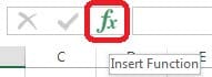
Formula.
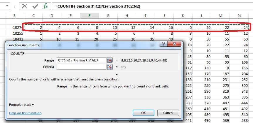
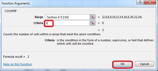
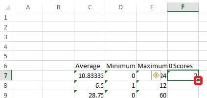
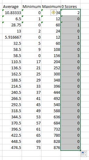
Count the number of 0 homework scores for each student.
Cell range F7:F29
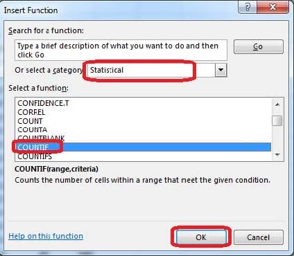
Use function COUNTIF
Range: all possible homework scores for each student on "Section 3" worksheet.
Criteria: 0
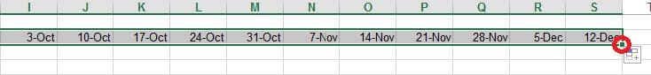
Modify the cell format to date.
Cell range C2:S2
Type: 14-Mar
Locale (location): English (United States)


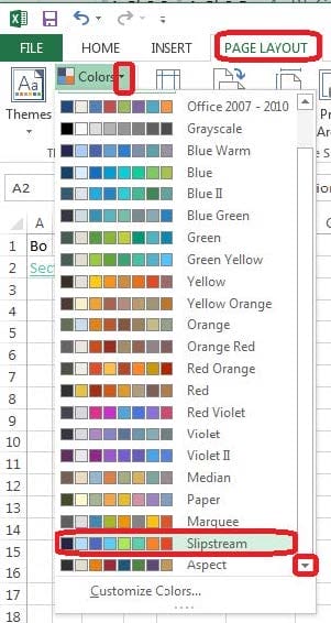
Add conditional formatting.
Color Scales: Green –White-Red Color Scale
Midpoint: Percentile, "70"
Maximum: Number, "25"


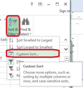
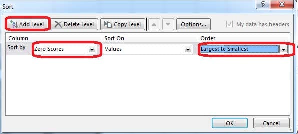
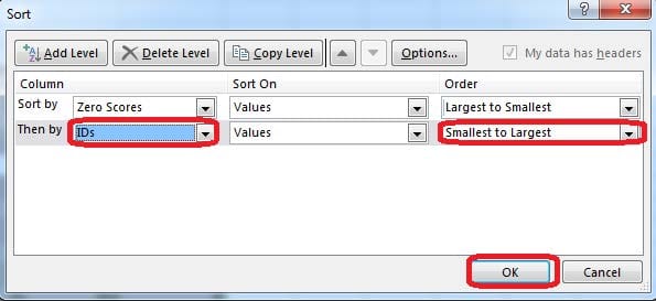
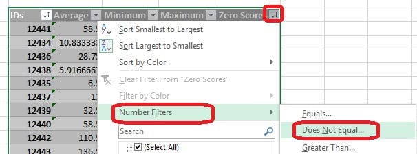
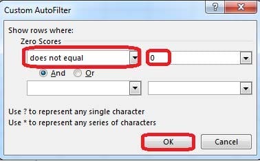
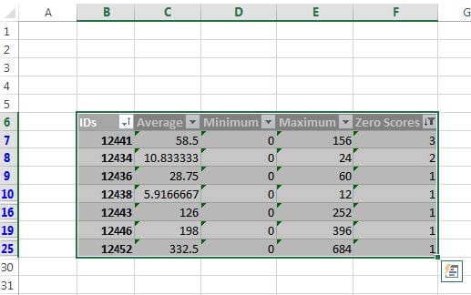
Sort and Filter. Apply a sort and a filter to the table. Cell range B6:F29 Sort Column Zero Scores Order Largest to Smallest Column IDs Order Smallest to Largest Filter Hide students ids with no zero scores.
Formula.
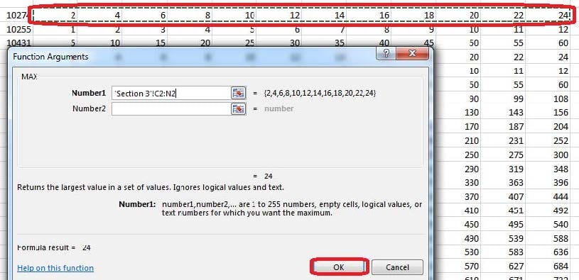
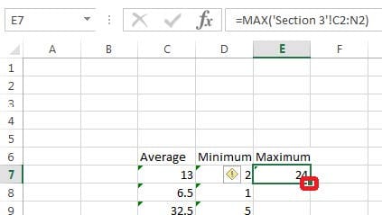
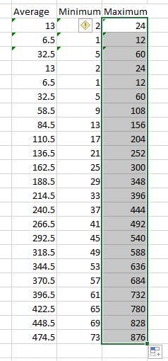
Find themaximum homework score for each student.
Cell rangeE7:E29
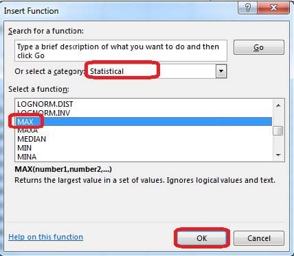
Use Function MAX
Number 1: maximum homework score for each student on "Section 3" worksheet.
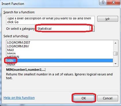
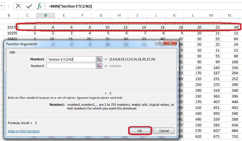
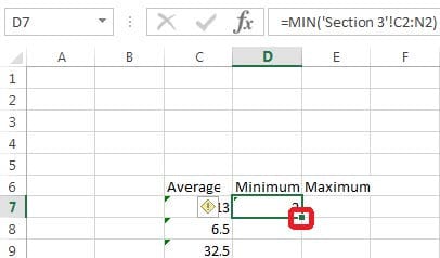
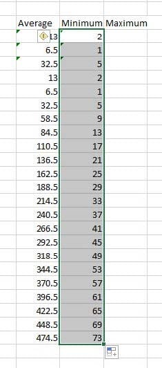
Formula.
Find the minimum homework score for each student.
Cell range D7:D29
Number 1: minimum homework score for each student on "Section 3" worksheet.

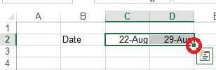
Add a header and the date for each of the columns (assignments) in the range.
Cell B2.
Text "Date".
Cell Range C2: S2
Text: "22-Aug, 29-Aug,