Exam2pass
0 items Sign In or Register
  • Home
  • IT Exams
  • Guarantee
  • FAQs
  • Reviews
  • Contact Us
  • Demo
Exam2pass > Microsoft > Microsoft Certifications > 77-727 > 77-727 Online Practice Questions and Answers

77-727 Online Practice Questions and Answers

Questions 4

SIMULATION

Project 1 of 7: Tailspin Toys

Overview

You recently opened an online toy store. You have sold products to 500 individual customers. You are evaluating customer data and order data.

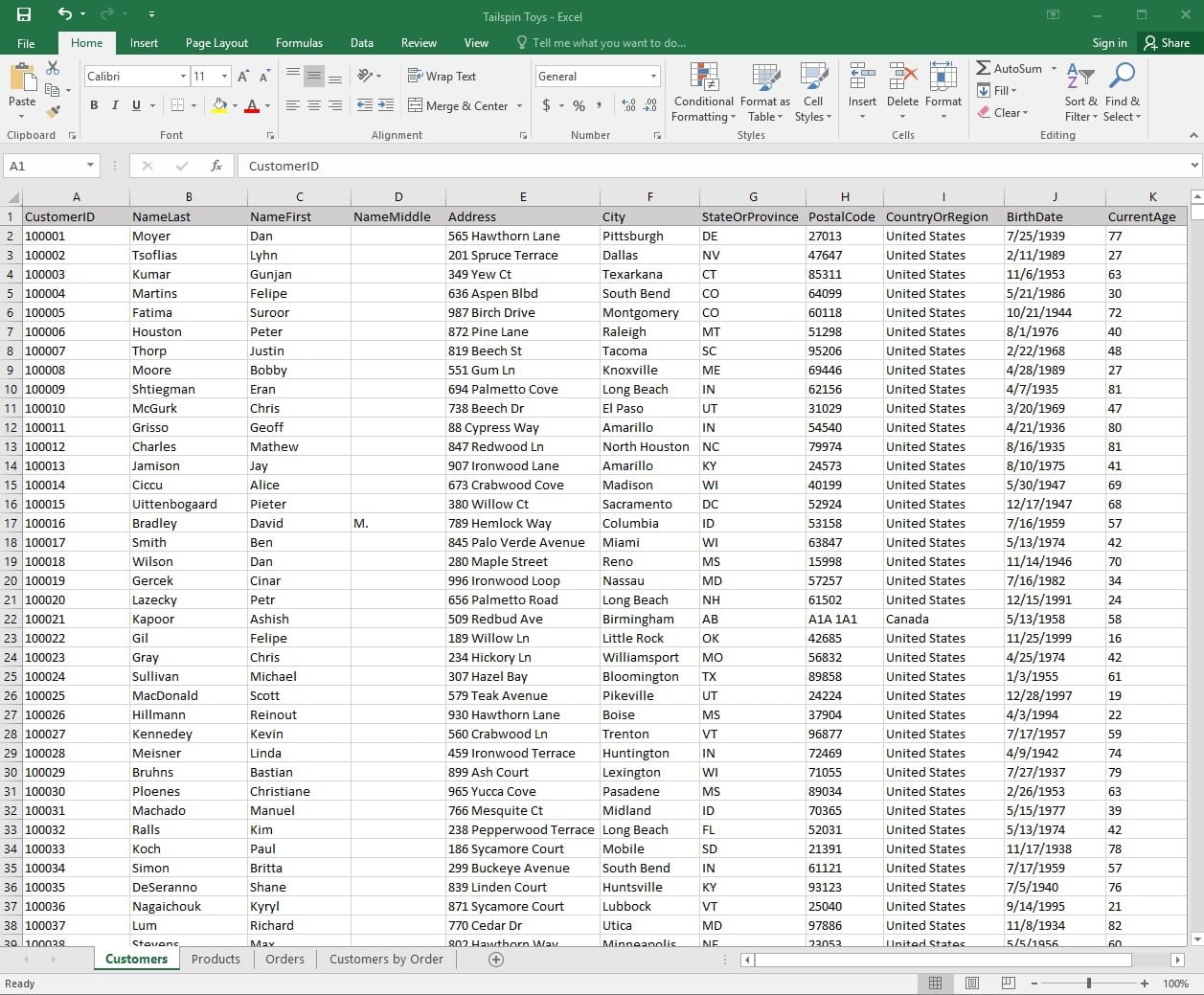
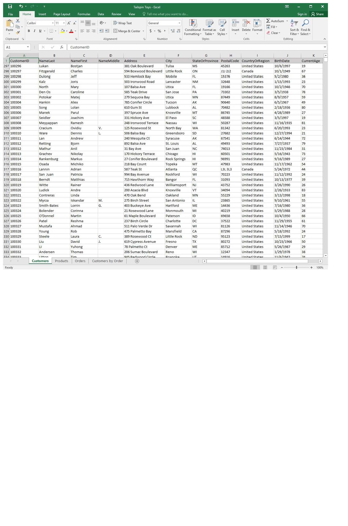
On the “Customers” worksheet, enter a formula in cell N2 that uses an Excel function to return the average age of the customers based on the values in the “CurrentAge” column.

Buy Now

Correct Answer: See explanation below.

Explanation:

1.

Select cell N2 on the “Customers” worksheet, which is where you want the Excel function to return the result to.

2.

In the Address bar, type the average function syntax; =AVERAGE(K1:K101).

References:

https://support.office.com/en-us/article/AVERAGE-function-047BAC88-D466-426C-A32B-8F33EB960CF6

Questions 5

SIMULATION

Project 2 of 7: Donor List Overview

You are an executive assistant for a non-profit organization named Bellows College. You are updating a workbook containing lists of donors.

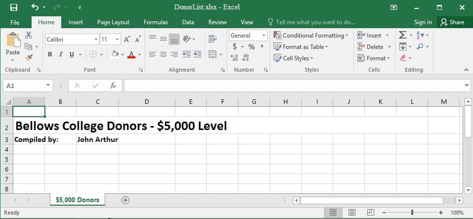
On the “$5,000 Donors” worksheet, hyperlink cell C3 to the email address “john@bellowscollege.com”.

Buy Now

Correct Answer: See explanation below.

Explanation:

1.

Click on cell C3.

2.

Enter the following formula: “=HYPERLINK(john@bellowsollege.com, C3)

References:

https://support.office.com/en-us/article/HYPERLINK-function-333C7CE6-C5AE-4164-9C477DE9B76F577F

Questions 6

SIMULATION

Project 3 of 7: Tree Inventory

Overview

You are updating the inventory worksheet for a local tree farm.

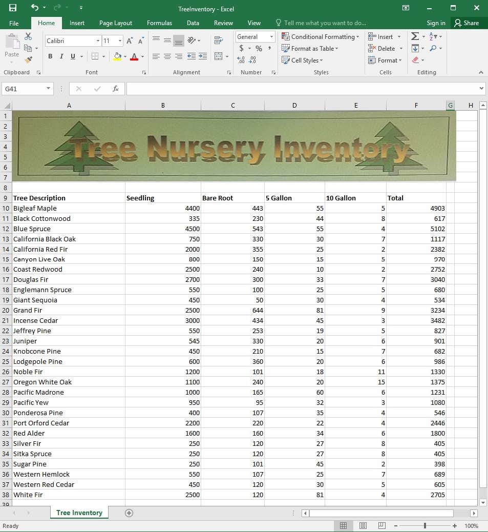
Change the margins to 1.0’’ (2.54 cm) on the top and bottom, 0.75’’ (1.90 cm) on the left and right, with a 0.5’’ (1.27 cm) header and footer.

Buy Now

Correct Answer: See explanation below.

Explanation:

1.

Select the worksheet you want to apply the margin changes to.

2.

Select Margins in the Page Setup group from the Page Layout tab.

3.

Click Custom Margins, then in the Top and Bottom dialog box enter 1.0’’ (2,54cm), in the Left and Right dialog box enter 0.75’’(1.90cm), and enter 0.5’’(1.27cm) in the Header and Footer dialog box.

References:

https://support.office.com/en-us/article/Set-page-margins-before-printing-a-worksheet-353F52FC-0D2C4958-9166-99FBD22B963A

Questions 7

SIMULATION

Project 3 of 7: Tree Inventory Overview

You are updating the inventory worksheet for a local tree farm.

Check the spreadsheet for accessibility problems. Correct the error by adding “Tree Nursery Inventory” as an alternative text file. You do not need to fix the warning.

Buy Now

Correct Answer: See explanation below.

Explanation:

1.

To check the accessibility select the Review tab from the ribbon.

2.

Select Check Accessibility.

3.

Review the results.

4.

Exit the Accessibility Checker.

5.

Right-click on the worksheet then click Format and then click Alt Text.

6.

Type “Tree Nursery Inventory” in the Description box.

7.

Click OK.

References:

https://support.office.com/en-us/article/Use-the-Accessibility-Checker-to-find-accessibility-issuesa16f6de0-2f39-4a2b-8bd8-5ad801426c7f

Questions 8

SIMULATION

Project 4 of 7: Car Inventory

Overview

You manage the office of a used car business. You have been asked to prepare the inventory list for a big annual sale.

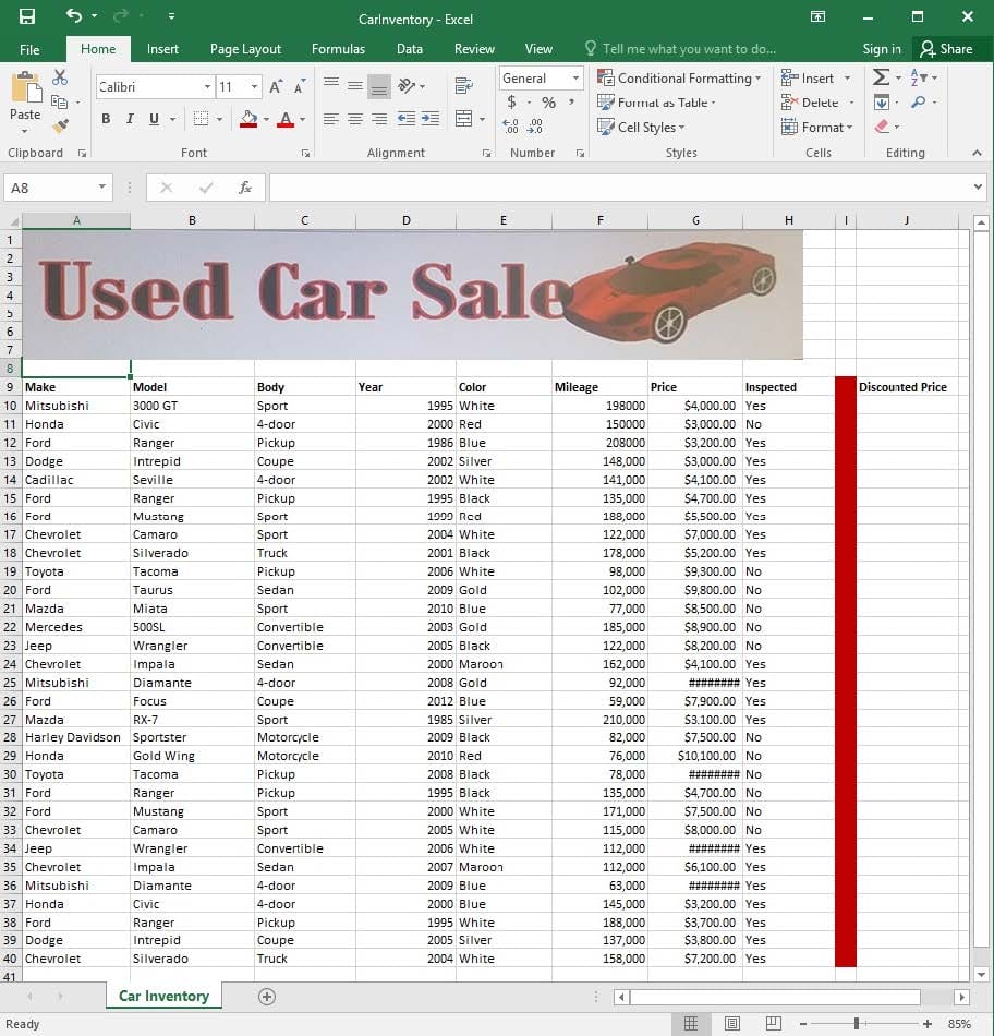
Apply the Rose, Table Style Light 17 (Table Style Light 17) to the “Inventory” table.

Buy Now

Correct Answer: See explanation below.

Explanation:

1.

On the “Inventory” table, click on any cell.

2.

Click on Format as Table from the Home tab.

3.

Select the Rose, Table Style Light 17 as desired.

References:

https://support.office.com/en-us/article/Format-an-Excel-table-6789619F-C889-495C-99C22F971C0E2370

Questions 9

SIMULATION

Project 5 of 7: City Sports Overview

The city events manager wants to analyze the enrollment changes over the past five years for various adult and youth sports programs. You have been tasked to prepare tables for the analysis.

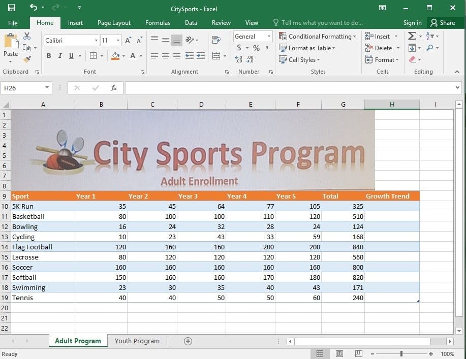
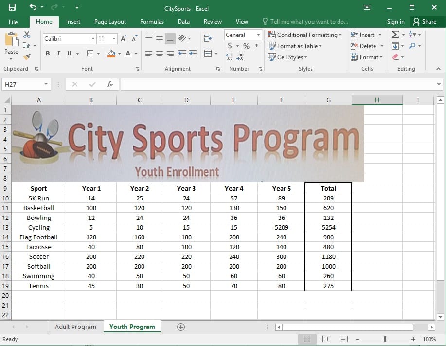
On the “Adult Program” worksheet, insert a Column sparkline for each sport that shows the enrollment for the past five years.

Buy Now

Correct Answer: See explanation below.

Explanation:

1.

On the “Adult Program” worksheet, select the area you want the sparkline to be inserted.

2.

Click Column in the Sparklines group from the Insert tab.

3.

Enter the range of cells in the Data Range box, in this case A10:A19.

OR

3.

Select the range of cells by temporarily collapsing the dialog box and manually selecting the cells.

4.

Click OK and the Sparkline Tools will appear, the Design tab can be used to customize the sparklines.

References:

https://support.office.com/en-us/article/analyze-trends-in-data-using-sparklines-be6579cf-a8e3-471a-a459873614413ce1

Questions 10

SIMULATION

Project 5 of 7: City Sports

Overview

The city events manager wants to analyze the enrollment changes over the past five years for various adult and youth sports programs. You have been tasked to prepare tables for the analysis.

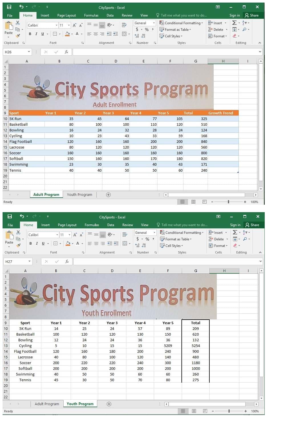
Unhide the “Summary” worksheet.

Buy Now

Correct Answer: See explanation below.

Explanation:

1. Select Format from the Home tab then choose Hide and Unhide then select Unhide. OR

1.

Hold on the Ctrl button on the keyboard and choose all the worksheet tabs then choose the Unhide option in the right menu.

2.

Click on the first worksheet tab, then hold down the Shift key on the keyboard as you click on the last worksheet tab, then choose the Unhide option.

OR

1.

From the View tab, click Custom Views in the Workbook Views group.

2.

Click the “Summary” view which is hidden, then click Show. References:

https://www.isunshare.com/blog/hide-or-unhide-sheets-in-excel-2016/

Questions 11

SIMULATION

Project 6 of 7: Bike Tours Overview

You are the owner of a small bicycle tour company summarizing trail rides that have been booked for the next six months.

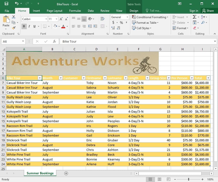
On the “Summer Bookings” worksheet, remove the table functionality from the table. Retain the cell formatting and location of the data.

Buy Now

Correct Answer: See explanation below.

Explanation:

1.

Click Design from the Ribbon on Table Tools.

2.

In the Tools group, click on Convert to Range.

OR

1. Right-click the table then click on Table then press Convert to Range.

References:

https://support.office.com/en-us/article/convert-an-excel-table-to-a-range-of-data-0b326ff1-1764-4ebe84ea-786265d41c77?redirectSourcePath=%252fen-us%252farticle%252fRemove-a-table-without-losingthe-data-or-table-format-ADF88635-90F5-4FAA-9417-19862F38CCE8andui=en-USandrs=en-USandad=US

Questions 12

SIMULATION

Project 6 of 7: Bike Tours Overview

You are the owner of a small bicycle tour company summarizing trail rides that have been booked for the next six months.

Insert page numbering in the center of the footer on the “Summer Bookings” worksheet using the format Page 1 of ?.

Buy Now

Correct Answer: See explanation below.

Explanation:

1. On the “Summer Bookings” worksheet, click Header and Footer from the Text group situation on the

Insert tab.

2.

Click Click to add footer which would display the Header and Footer tools which gets added to the Design tab.

3.

Specify where the page number should be by selecting the Center section box.

4.

On the Design tab in the Header and Footer Elements group, click Page Number.

5.

The placeholder and[Page] will appear in the selected section, to add the total number of pages type the word of followed by the space in the Header and Footer Elements group after clicking Number of Pages, then the placeholder and[Page] of and[Pages] appear.

6.

Click anywhere outside the header or footer area to display the page numbers in Page Layout View.

7.

Once you are done working in the Page Layout View, click Normal in the Workbook Views group situated on the View tab. OR You can also click Normal on the status bar.

References:

https://support.office.com/en-us/article/Insert-page-numbers-on-worksheets-27A88FB9-F54E-4AC4-84D7BF957C6CE29C

Questions 13

SIMULATION

Project 7 of 7: Farmers Market

Overview

You are the Director of a local farmers’ market. You are creating and modifying charts for a report which shows the amounts and variety of products sold during the season.

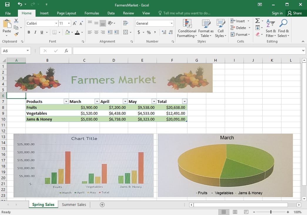
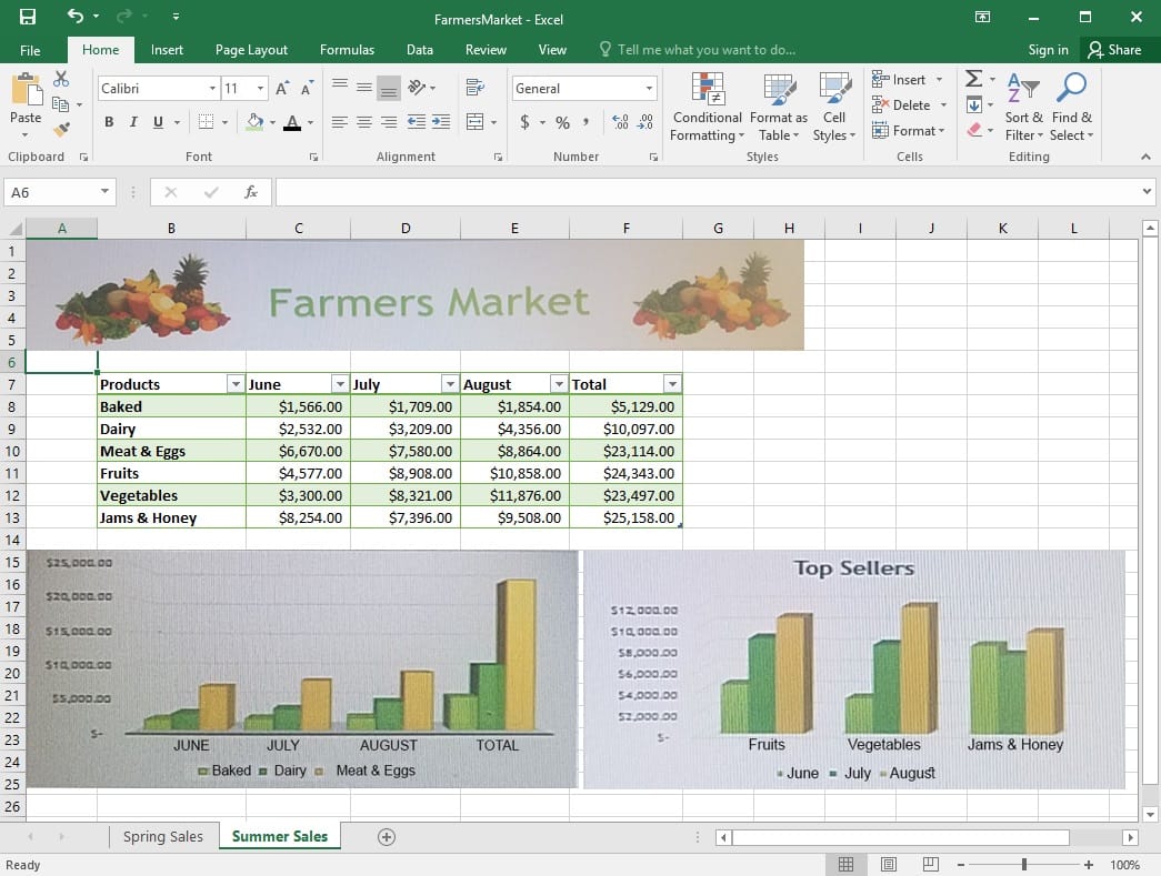
On the “Summer Sales” worksheet, use the data in the “Products” and “Total” columns only to create a 3-D Pie chart. Position the new chart to the right of the column charts.

Buy Now

Correct Answer: See explanation below.

Explanation:

1.

Select the data you would like to use, in this case it would be the data in the “Products” and “Total” columns from the “Summer Sales” worksheet.

2.

Click on Insert Pie Chart situation on the Insert tab then pick the 3-D Pie chart as desired.

3.

Format the chart as desired by using Chart Elements, the Chart Styles, or the Chart Filters.

4.

Drag the Pie Chart to the desired location which is to the right of the column charts.

References:

https://support.office.com/en-us/article/Add-a-pie-chart-1A5F08AE-BA40-46F2-9ED0-FF84873B7863

Exam Code: 77-727
Exam Name: Excel 2016 Core Data Analysis, Manipulation, and Presentation
Last Update: May 25, 2026
Questions: 35

PDF (Q&A)

$45.99
ADD TO CART

VCE

$49.99
ADD TO CART

PDF + VCE

$59.99
ADD TO CART

Exam2Pass----The Most Reliable Exam Preparation Assistance

There are tens of thousands of certification exam dumps provided on the internet. And how to choose the most reliable one among them is the first problem one certification candidate should face. Exam2Pass provide a shot cut to pass the exam and get the certification. If you need help on any questions or any Exam2Pass exam PDF and VCE simulators, customer support team is ready to help at any time when required.

Home | Guarantee & Policy |  Privacy & Policy |  Terms & Conditions |  How to buy |  FAQs |  About Us |  Contact Us |  Demo |  Reviews

2026 Copyright @ exam2pass.com All trademarks are the property of their respective vendors. We are not associated with any of them.